Introduction
The creative goal of this project was an attempt to tie together a number of themes that are of interest to me, and to use some of the physical computing skills that I have been learning to create an installation that would hopefully be beautiful and engaging.
The main theme in this project relates to an ongoing interest of mine into the nature of time, and it’s connection to the ancient Chinese system of divination the I Ching. A strongly interrelated theme here is an interest in systems which mimic the functioning of autotrophic organisms. These are organisms which nourish themselves, thus systems which mimic their functioning will involve some sort of iterative feedback loop to form a sort of auto-catalytic, self-reinforcing process. I became interested in this idea after seeing ‘Talysis II, Autotrophs’ by Paul Prudence in the book ‘Generative Design’ by Bohnacker et al. (page 104-107).
Talysis II from Paul Prudence on Vimeo.
To understand how autotrophism relates to theories of time, or more specifically non-western theories of time where time is considered to be cyclical, consider the picture below of the Ouroboros.
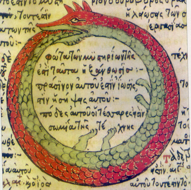
(Figure 1: The Ouroboros, Drawing by Theodoros Pelecanos, in the alchemical tract Synosius (1478).
“The Ouroboros often symbolizes self-reflexivity or cyclicality, especially in the sense of something constantly re-creating itself, the eternal return…” Source; wikipedia.org)
The western scientific view of time as a smooth surface, where this moment is just like the one before it, and just like the one about to occur, is an idea that this project aims to challenge.
The System
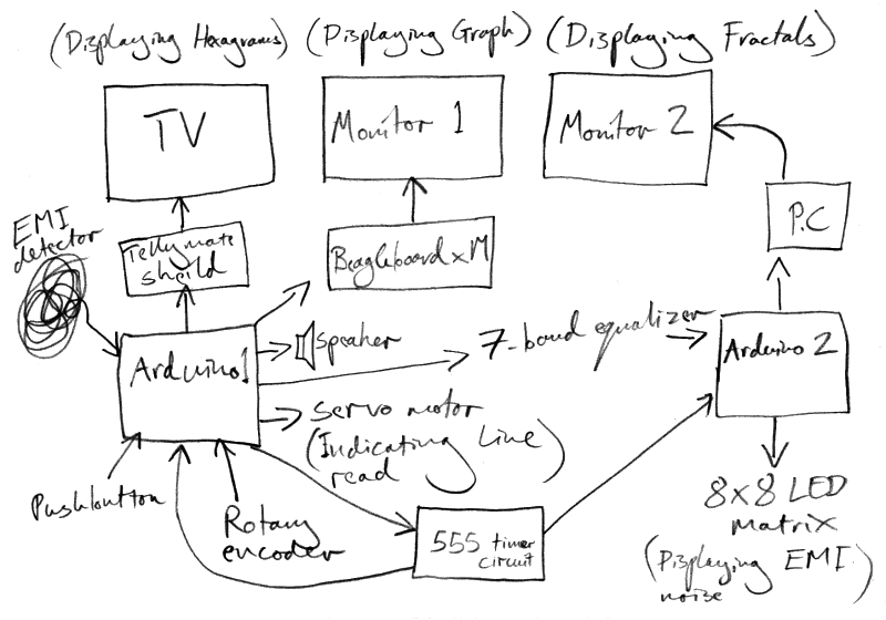
(Figure 2: System Overview.)
My explanation of how the system works will begin with the electromagnetic interference (EMI) detector. EMI is a form of electromagnetic radiation, this is a combination of electrical and magnetic waves travelling outward from anywhere that an electrical power signal is changing or being turned off and on rapidly. The antenna for detecting EMI here is simply a 3 foot length of solid core wire, connected to an analogue pin of Arduino 1, via an LM386 amplifier chip circuit.
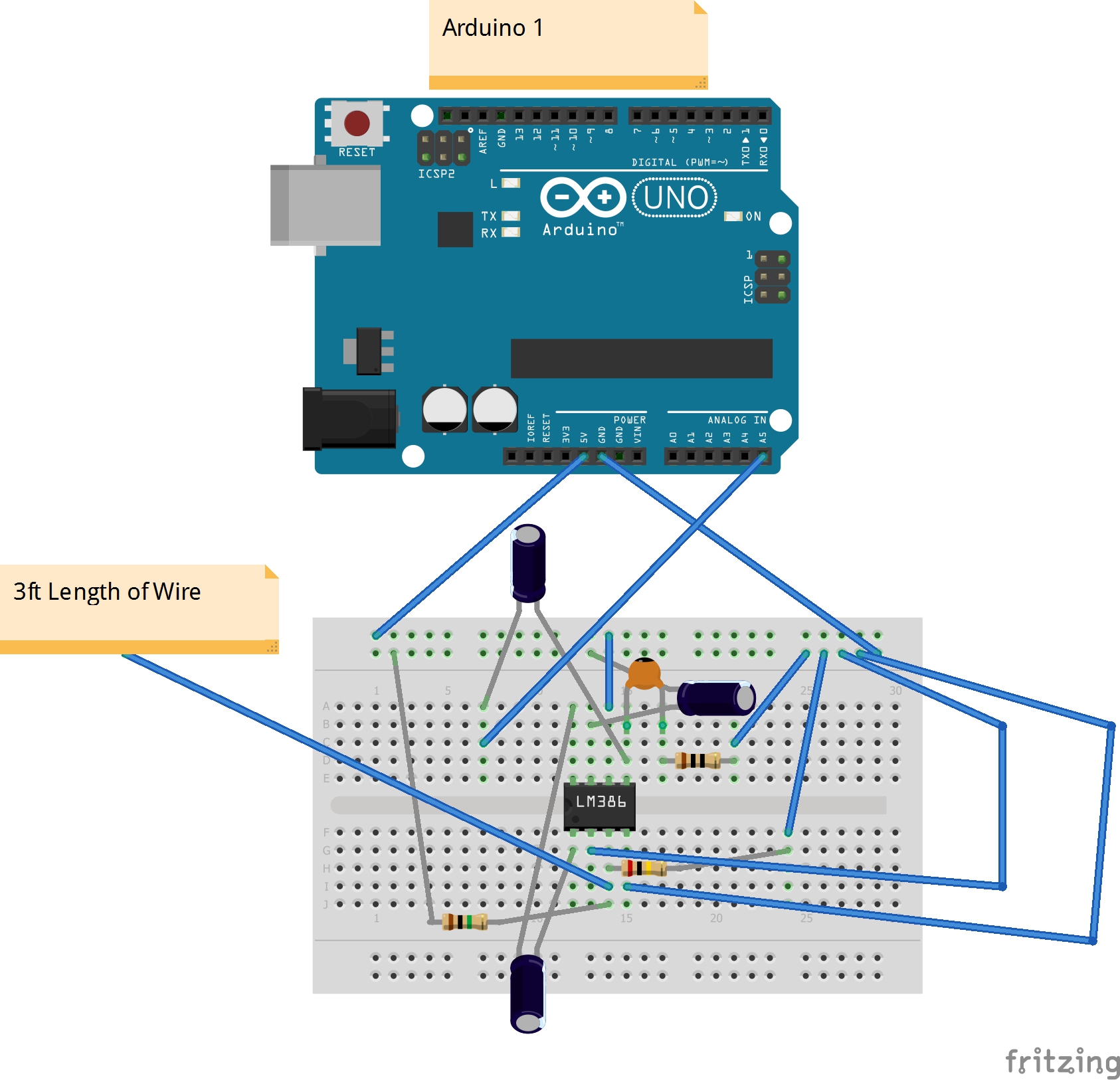
(Figure 3: EMI detector, breadboard view. Signal amplified with LM386 amplifier chip.)
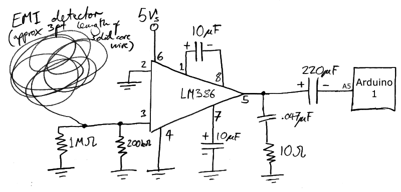
(Figure 4: EMI detector, schematic view. Signal amplified with LM386 amplifier chip.)
The system is listening for electromagnetic energy being emitted from various electronic devices in the local environment. Sometimes, an electrical device that has the potential to give off EMI is shielded to prevent interference from escaping; however a great many devices that emit EMI are shielded very lightly or not at all.
One unexpected autotrophic element of this system became apparent when I later added a servo motor right next to the wire antenna of the EMI detector. The values being read by the EMI detector determine whether or not the servo should move, and if so where. But every time the servo motor moves this creates a clearly perceptible change in the EMI detected, this was apparent by either looking at the values being read by the analogue pin on Arduino 1, or just listening to the tone being generated out of digital pin 11 on Arduino 1 (see figures 5 and 6), using the code below;
void loop() {

  int analIP = analogRead(aPiNoise);
  showDiag=0;
  if (minNoise>analIP) { minNoise=analIP; showDiag=0; }
  if (maxNoise<analIP) { maxNoise=analIP; showDiag=0; }
  if (opct < 1050 && showDiag) {     Serial.print(" no: "); Serial.print(minNoise); Serial.print(" "); Serial.print(maxNoise);     if (++opct % 12 != 0) Serial.print(" "); else Serial.println("");   }   if (abs(currAnal-analIP)>10) {
    currAnal=analIP;
    totAnal += currAnal;

    if (muteState)
      noTone(spkrPin);
    else
      tone(spkrPin, map(currAnal, minNoise, maxNoise, 30, 10000), 200);  // pin, Hz, mS

  }

(Figure 5: Speaker and amplifier, breadboard view. Signal amplified with LM386 amplifier chip.)
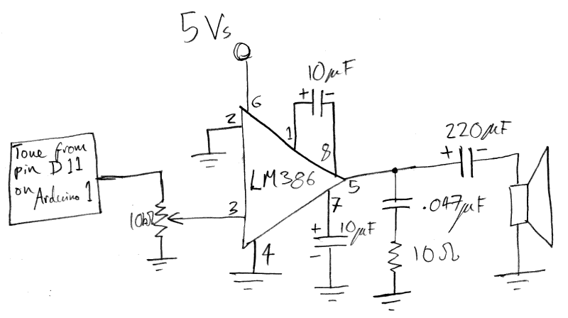
(Figure 6: Speaker and amplifier, schematic view. Signal amplified with LM386 amplifier chip.)
The EMI values being read by Arduino 1 on analogue pin 5 are used to generate the lines (or yao) of an I Ching hexagram. Before I explain how this is done, I will first describe one of the traditional methods for casting the I Ching; the throwing of three coins. The lines of an I Ching hexagram are either;
⦁ Old Yin (—X—)
⦁ Young Yang (———)
⦁ Young Yin (— —)
⦁ Old Yang (—θ—)
For the three coins method, we give the lines the following values;
⦁ 6 = Old Yin (—X—)
⦁ 7 = Young Yang (———)
⦁ 8 = Young Yin (— —)
⦁ 9 = Old Yang (—θ—)
And we say that a tails = 2, and heads = 3. Then when throwing three coins;
⦁ Three tails = 6 = Old Yin (—X—)
⦁ Two tails and one head = 7 = Young Yang (———)
⦁ Two heads and one tail = 8 = Young Yin (— —)
⦁ Three heads = 9 = Old Yang (—θ—)
Thus there is a 1/8 chance of throwing a 6, a 1/8 chance of throwing a 9, a 3/8 chance of throwing a 7, and a 3/8 chance of throwing an 8.
What we have streaming from our EMI detector is a constant flow of noise data (values between 0 and 1023). To replicate the throwing of three coins we take the values being read by the EMI detector and sum them every time the value changes by 10 or more.
Every time Arduino 1 receives a flash from the 555 timer circuit, the summed value is converted to a binary number. The equivalent now of throwing three coins is to take the least significant three bits of this binary number and apply the following rules;
⦁ 000 = Old Yin (—X—)
⦁ 001, 010, 011 = Young Yang (———)
⦁ 100, 101, 110 = Young Yin (— —)
⦁ 111 = Old Yang (—θ—)
The lines and resulting hexagrams are displayed on a black and white CRT monitor using a TellyMate shield. Hexagrams are drawn from the bottom up.
The rate at which these snapshot readings are taken is determined by rate of oscillation of the 555 timer circuit below;
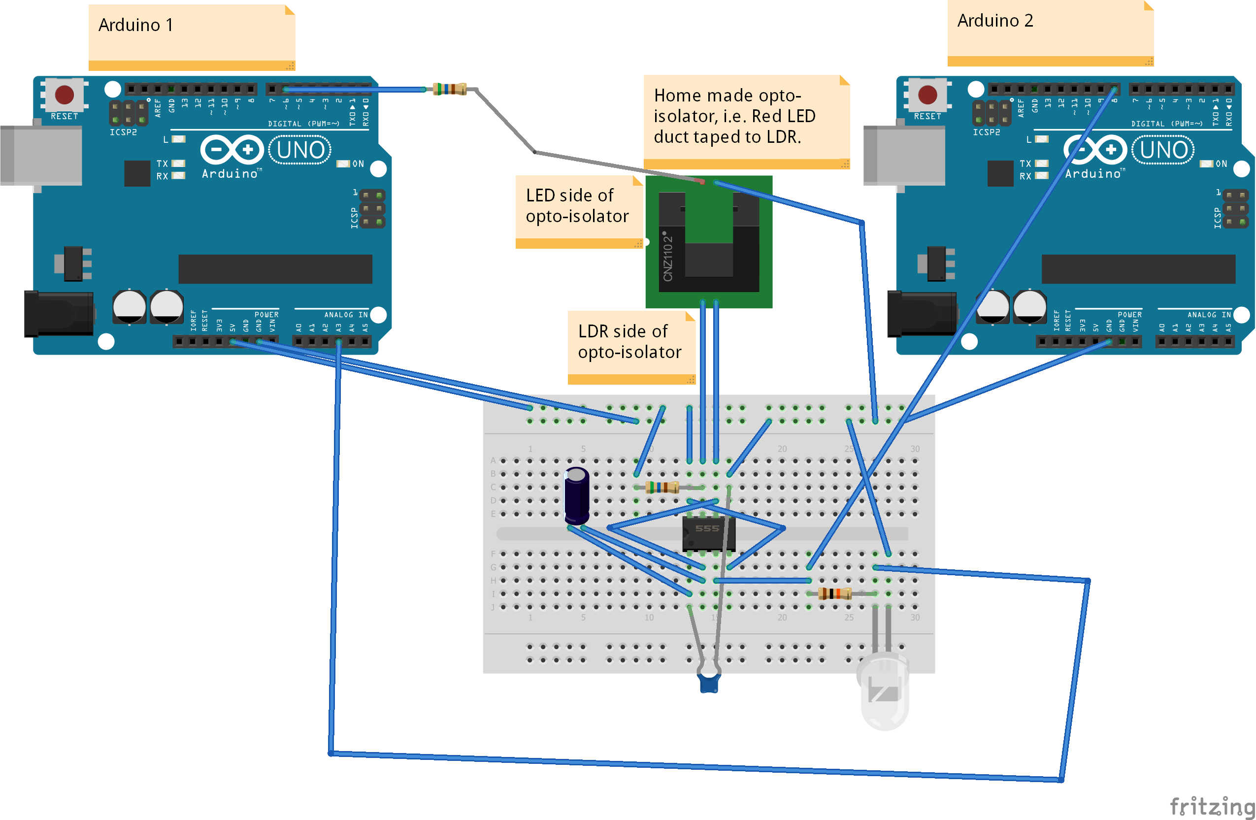
(Figure 7: 555 timer and opto-isolator circuit, breadboard view.)
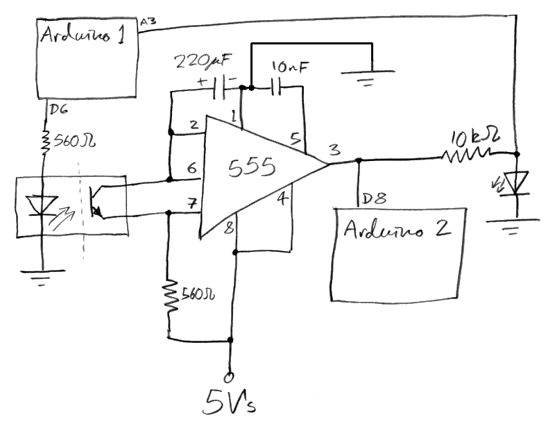
(Figure 8: 555 timer and opto-isolator circuit, schematic view.)
Between pin 6 and 7 of the 555 timer chip in the above schematic is a home made opto-isolator. This is a red LED duct taped to an light dependent resistor (LDR);
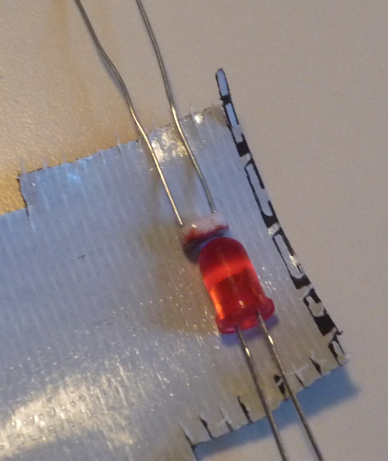
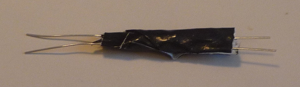
Opto-isolators are normally used to enable the transfer of data over wide voltage differences. There was not actually any need for me to have used one here, but I just like the idea of them.
The anode of the LED side of the opto-isolator is connected to digital pin 6 on Arduino 1, this pin is capable using pulse width modulation (PWM) to vary the brightness of the LED. By experimenting with different PWM values using the analogWrite() function on Arduino 1, I found that the range of values 1 to 64 gave a reasonable range of speeds of oscillation. It occurred to me a strange synchronicity that the values 1 to 64 would fit so nicely here. There are 64 possible hexagrams in the I Ching, and each has its own number from 1 to 64 ordered in a sequence known as the King Wen sequence;
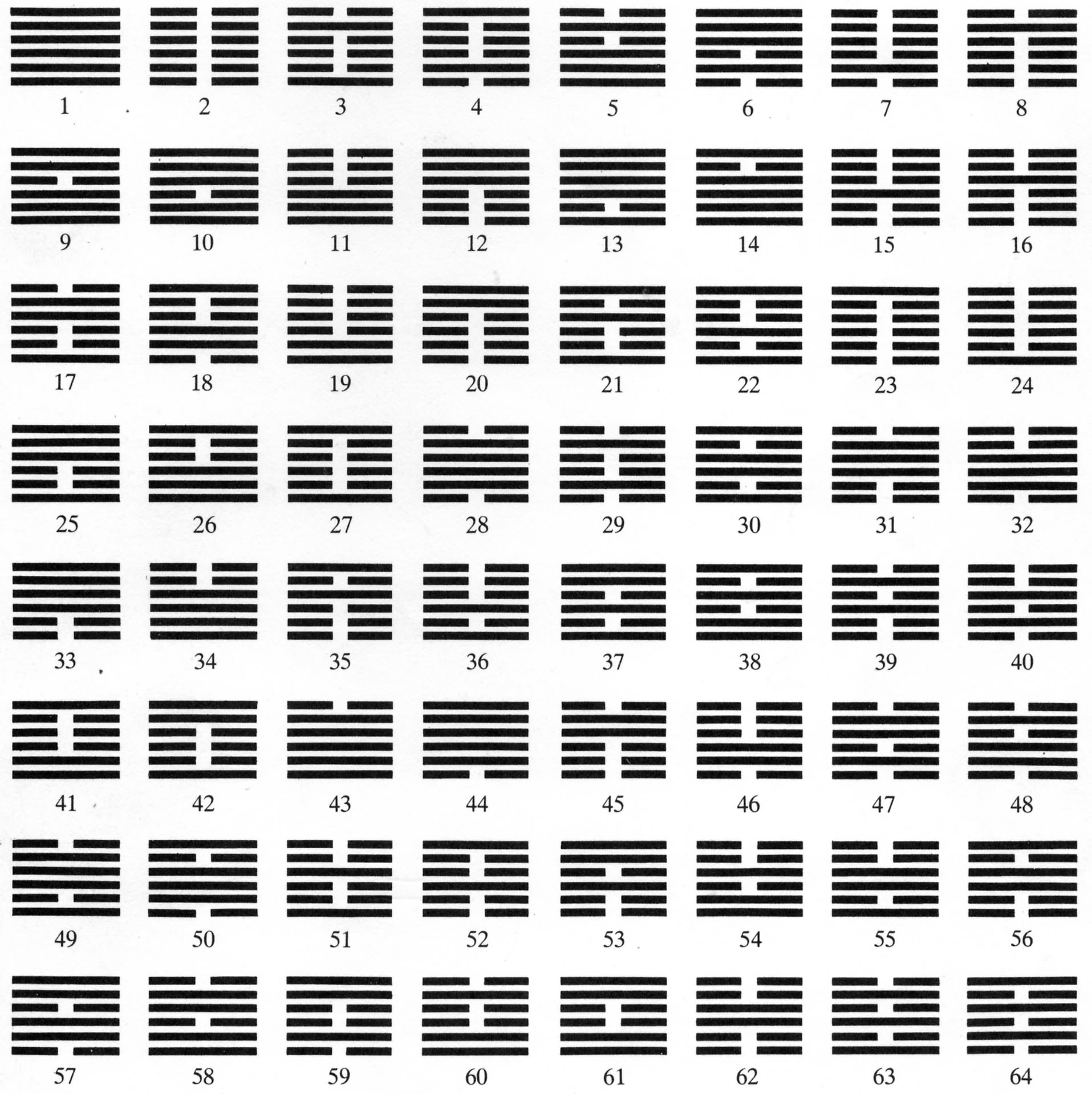
(Figure 9: The King Wen Sequence. Source; http://fractalenlightenment.com/14061/enlightening-video/mckenna-and-bradens-fractal-nature-of-time)
The designed autotrophic element of the system occurs here; once a hexagram is generated the number of that hexagram from the table above determines the brightness of the LED in the opto-isolator, which in turn determines the rate at which the EMI noise is sampled to determine the next hexagram, which itself then determines the brightness of the LED for the next hexagram, ad infinitum.
As a way of visually demonstrating the process at work here, that of taking a snapshot of noise data. I took the EMI tone generated by pin 11 of Arduino 1, and passed it through a 7 band graphic equaliser display filter chip (the MSGEQ7, using this library and these instructions), the output from the MSGEQ7 is being passed to Arduino 2;
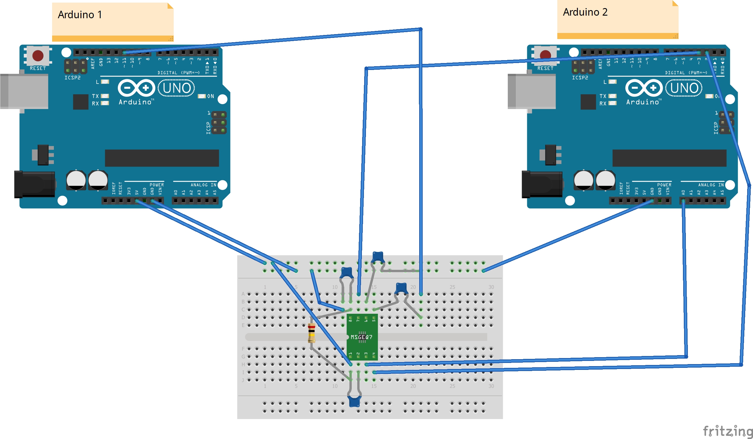
(Figure 10: 7-band equalizer circuit, breadboard view.)

(Figure 11: 7-band equalizer circuit, schematic view.)
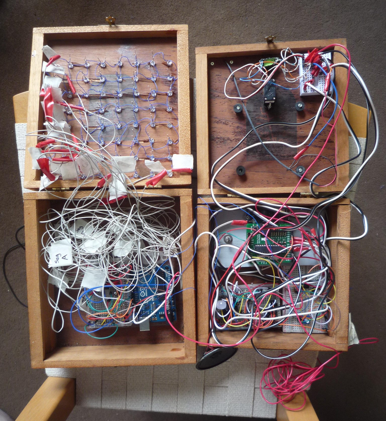
Also connected to Arduino 2 is an 8×8 matrix of blue LEDs being controlled via a MAX7219 driver chip (using this library, and these instructions);

(Figure 12: 8×8 LED matrix controlled via MAX7219 chip, breadboard view.)

(Figure 13: 8×8 LED matrix controlled via MAX7219 chip, schematic view.)
The left-most column of the 8×8 matrix indicates the sampling rate by pulsing from the central rows outwards. While the remaining 7 columns indicate the 7 bands of the EMI noise once it has been passed through the MSGEQ7 circuit, this is demonstrated to the video here;
Workshops In Creative Coding 2 Project Demo from George Haworth on Vimeo.
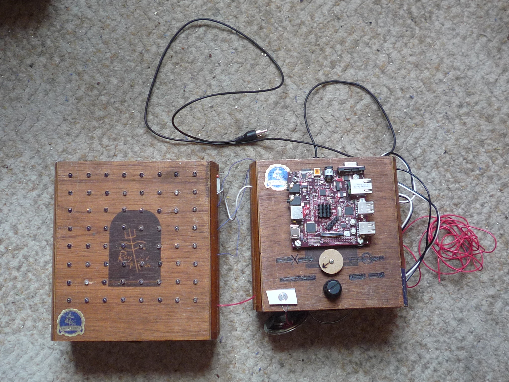
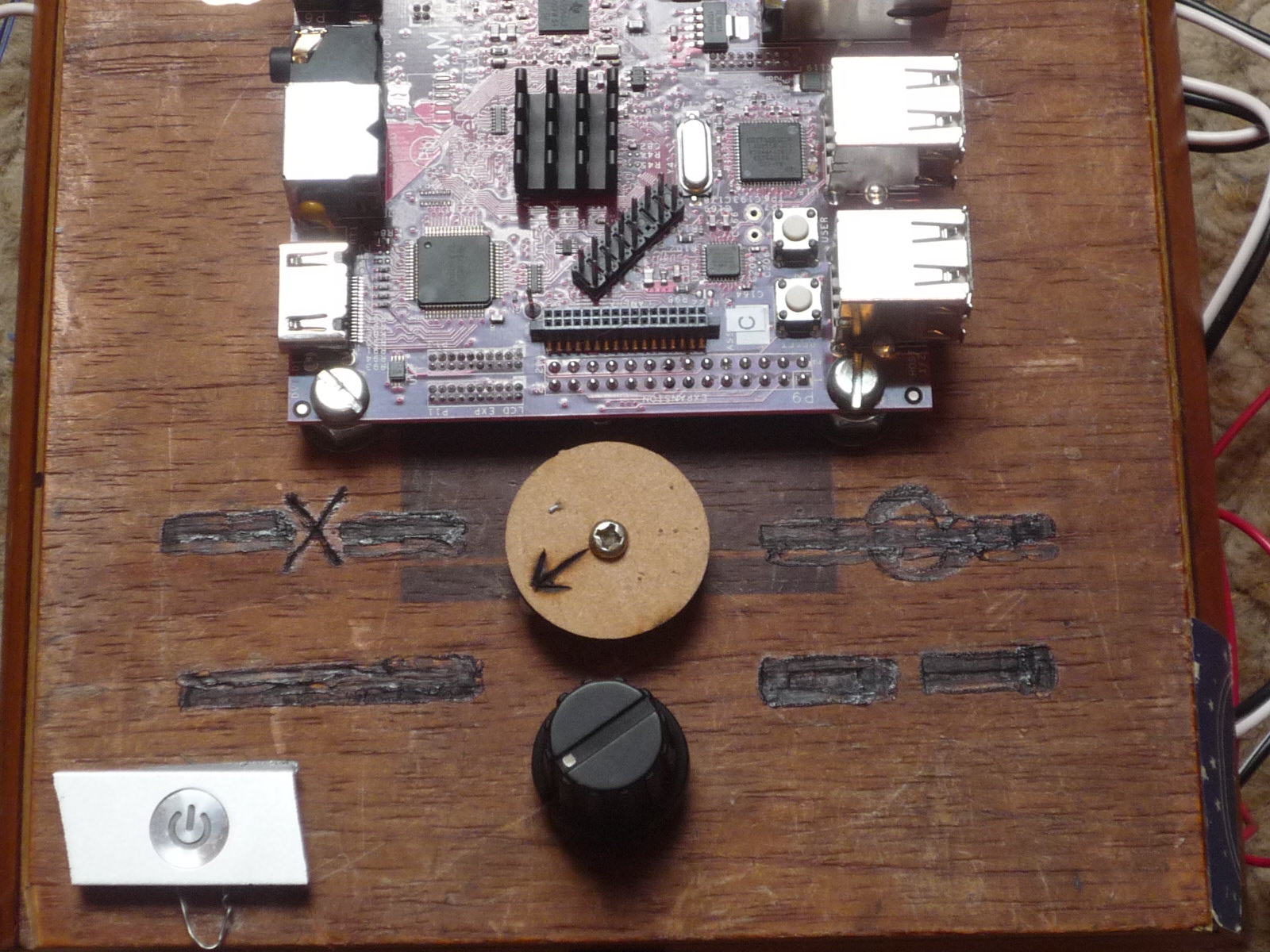
On the above video, you can also see that I have attached a servo motor to the top of the old cigar box where Arduino 1 is housed. This servo motor has a disc with an arrow attached to it which points to a symbol to indicate the line that is currently being generated by the system (i.e. Old Yang, Young Yin, etc). The line symbols I drew on the old cigar box with a pyrography iron. There is also a push-button salvaged from an old PowerBook G4, and a rotary encoder with a push-button built into the cigar box. The top of another old cigar box forms the surface for the 8×8 LED matrix, and this box houses Arduino 2;
The servo motor, push-button, and rotary encoder are wired up as follows;
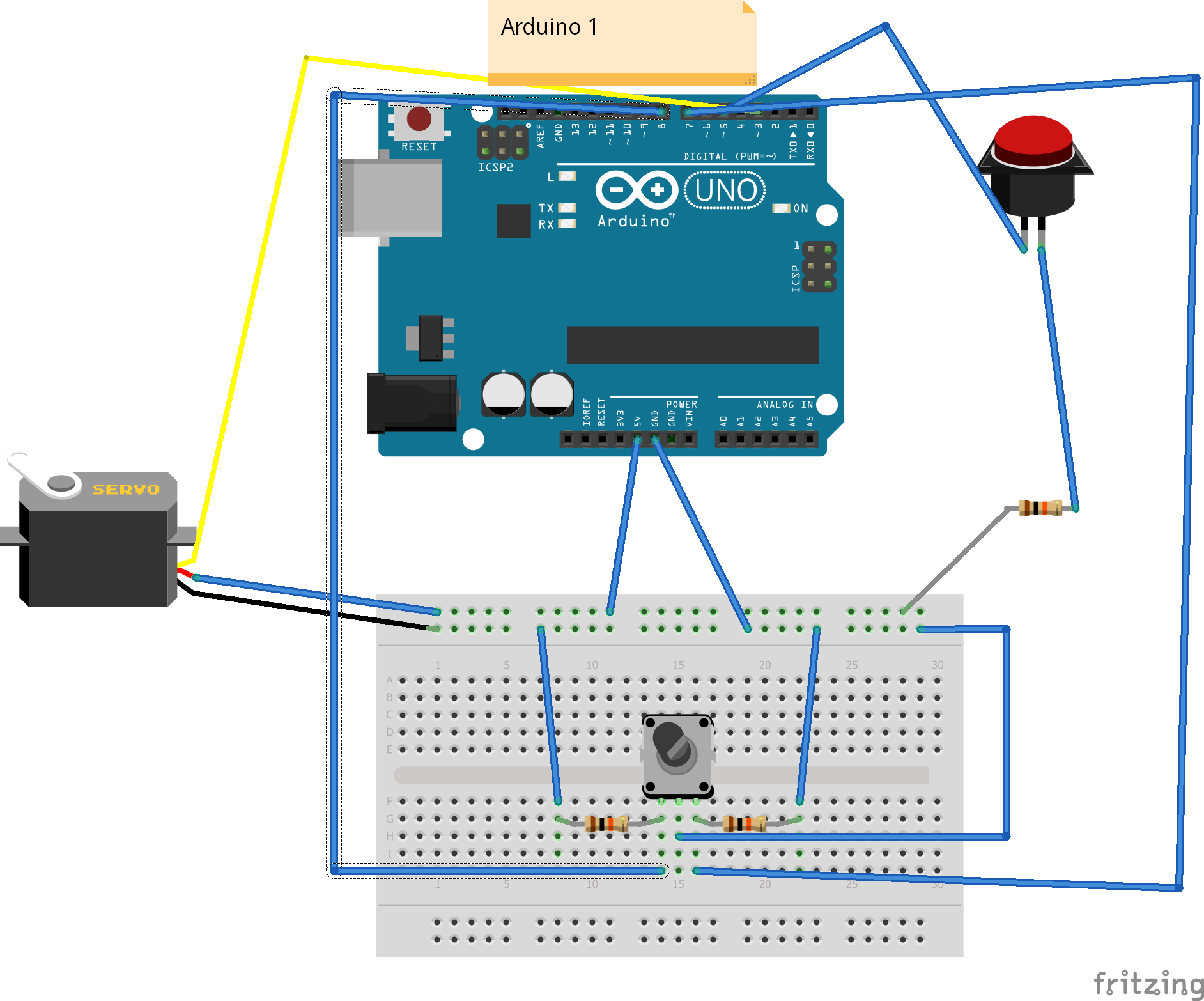
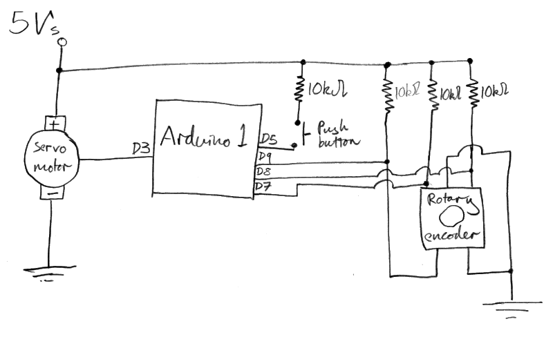
(Figure 14: Servo motor, rotary encoder and push-button, breadboard view.)(Figure 15: Servo motor, rotary encoder and push-button, schematic view.)
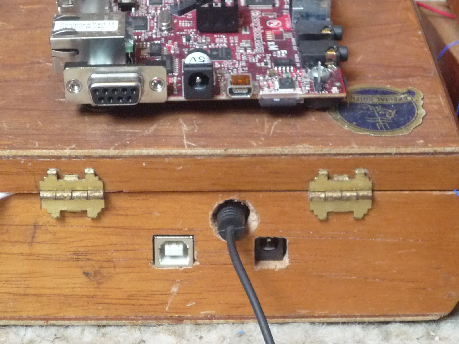
On top of the cigar box housing Arduino 1 is mounted a Beagleboard xM running Debian. I managed to install Processing on this by modifying these instructions for installing it on a Raspberry Pi, a Beagleboard was chosen over a Raspberry Pi due to the fact that it is slightly faster. A monitor was attached to the Beagleboard, on which is displayed the rising and falling values of temporal flux on the y-axis, against time on the x-axis. The idea of temporal flux is taken from ‘The Invisible Landscape’ by Terence McKenna, Chapter 1o includes a full explanation of this idea, and derivation of the values in Table 1 below.
For our purposes here, if we consider the King Wen sequence (Figure 9). We have 6 x 64 (=384) lines, or yao in the King Wen sequence. If we consider the bottom line of hexagram 1 to be the first yao, the top line of hexagram 1 to be the sixth yao, the bottom line of hexagram 2 to be the seventh yao, … , and the top line of hexagram 64 to be the 384th yao. According to McKenna, these lines have a value for temporal flux (also termed novelty) associated with them, the 384 values for temporal flux associated with the 384 values of the King Wen sequence are presented in the table below;
0, 0, 0, 2, 7, 4, 3, 2, 6, 8, 13, 5, 26, 25, 24, 15, 13, 16, 14, 19, 17, 24, 20, 25, 63, 60, 56, 55, 47, 53, 36, 38, 39, 43, 39, 35, 22, 24, 22, 21, 29, 30, 27, 26, 26, 21, 23, 19, 57, 62, 61, 55, 57, 57, 35, 50, 40, 29, 28, 26, 50, 51, 52, 61, 60, 60, 42, 42, 43, 43, 42, 41, 45, 41, 46, 23, 35, 34, 21, 21, 19, 51, 40, 49, 29, 29, 31, 40, 36, 33, 29, 26, 30, 16, 18, 14, 66, 64, 64, 56, 53, 57, 49, 51, 47, 44, 46, 47, 56, 51, 53, 25, 37, 30, 31, 28, 30, 36, 35, 22, 28, 32, 27, 32, 34, 35, 52, 49, 48, 51, 51, 53, 40, 43, 42, 26, 30, 28, 55, 41, 53, 52, 51, 47, 61, 64, 65, 39, 41, 41, 22, 21, 23, 43, 41, 38, 24, 22, 24, 14, 17, 19, 52, 50, 47, 42, 40, 42, 26, 27, 27, 34, 38, 33, 44, 44, 42, 41, 40, 37, 33, 31, 26, 44, 34, 38, 46, 44, 44, 36, 37, 34, 36, 36, 36, 38, 43, 38, 27, 26, 30, 32, 37, 29, 50, 49, 48, 29, 37, 36, 10, 19, 17, 24, 20, 25, 53, 52, 50, 53, 57, 55, 34, 44, 45, 13, 9, 5, 34, 26, 32, 31, 41, 42, 31, 32, 30, 21, 19, 23, 43, 36, 31, 47, 45, 43, 47, 62, 52, 41, 36, 38, 46, 47, 40, 43, 42, 42, 36, 38, 43, 53, 52, 53, 47, 49, 48, 47, 41, 44, 15, 11, 19, 51, 40, 49, 23, 23, 25, 34, 30, 27, 7, 4, 4, 32, 22, 32, 68, 70, 66, 68, 79, 71, 43, 45, 41, 38, 40, 41, 24, 25, 23, 35, 33, 38, 43, 50, 48, 18, 17, 26, 34, 38, 33, 38, 40, 41, 34, 31, 30, 33, 33, 35, 28, 23, 22, 26, 30, 26, 75, 77, 71, 62, 63, 63, 37, 40, 41, 49, 47, 51, 32, 37, 33, 49, 47, 44, 32, 38, 28, 38, 39, 37, 22, 20, 17, 44, 50, 40, 32, 33, 33, 40, 44, 39, 32, 32, 40, 39, 34, 41, 33, 33, 32, 32, 38, 36, 22, 20, 20, 12, 13, 10
Table 1: The 384 Temporal Flux Values of the King Wen Sequence (Source; ‘The Invisible Landscape’ by Terence McKenna. Pages 162-163).
The rotary encoder functions to allow the viewer to observe this graph over longer or shorter periods of time. The notion that this graph aims to evoke is the idea that time can be described in much the same way as a stock market, as a series of rising and falling fluctuations of novelty. Where this moment is different from the one before it, and different from the one about to occur.
Attached to Arduino 2 is a PC running Ubuntu with Processing installed, the monitor attached to this PC is displaying fractal imagery adapted from here and created in Processing. I originally intended to display both the fractal imagery and the temporal flux graph on the Beagleboard, and have the push-button on the rotary encoder toggle between the two. However I found that the Beagleboard was unable to display the fractal images at an acceptable size and definition, therefore I chose to display the graph on the Beagleboard and the fractals on a PC.
Originally it had been planned that the fractal generation would be based on the hexagram number (King Wen sequence). However, when I realized that I would have to display the fractals on a PC instead of the Beagleboard, I could not see an immediate way to send the serial output from Arduino 1 to both the Beagleboard and the PC simultaneously, so a different approach was taken.
The 555 timer circuit (Figures 7 and 8) is connected to Arduino 2, the output from this is used in this case to let the PC know when a line is drawn. For a random number as input to the fractal generating sketch the summed value of the 7 bands of the MSGEQ7 circuit is taken and mapped to a range of values previously determined to produce interesting fractal images. To synchronise the generation of fractal images on one screen with the generation of hexagrams on the CRT screen, I looked at the time interval between the arrival of a flash from the 555 circuit. When I note that this interval had changed by more than 50%, I take this to indicate the start of a new hexagram.
Aside from the fact that the generated fractals are quite often very beautiful, the notion I am attempting to evoke by including them in the installation is the suggestion that time may be thought of as some sort of convoluted surface, or topological manifold. Where some regions of this surface are fairly uninteresting, and then the surface suddenly takes on a beautiful and fascinating pattern. Much the same way as how the felt experience of our lives often seems to be periods of stagnation, frustration and boredom interlaced with breakthrough moments, epiphanies and important revelations.
The great work continues…
Source Code
- Arduino sketch running on Arduino 1 is found here.
- Arduino sketch running on Arduino 2 is found here.
- Processing sketch running on Beagleboard xM is found here.
- Processing sketch running on PC is found here.
References and Acknowledgements
- ‘Talysis II, Autotrophs’ by Paul Prudence taken from the book ‘Generative Design’ by Bohnacker et al. (page 104-107).
- EMI detector idea taken from ‘Environmental Monitoring with Arduino: Building Simple Devices to Collect Data About the World Around Us‘ by Gertz et al. (Chapter 4.)
- Values for Temporal Flux taken from ‘The Invisible Landscape’ by Terence McKenna (pages 162-163), a full derivation of these values is explained in Chapter 10.
- Idea for homemade opto-isolator taken from ‘Handmade Electronic Music’ by Nicolas Collins. Page 181. (My favourite book at the moment!).
- Fractal idea adapted from; http://glsl.heroku.com/e#16063.0, and inspired by http://www.fractalforums.com/new-theories-and-research/very-simple-formula-for-fractal-patterns/
- Breadboard diagrams created using Fritzing.
- Project title from ‘Finnegans Wake’ by James Joyce.